

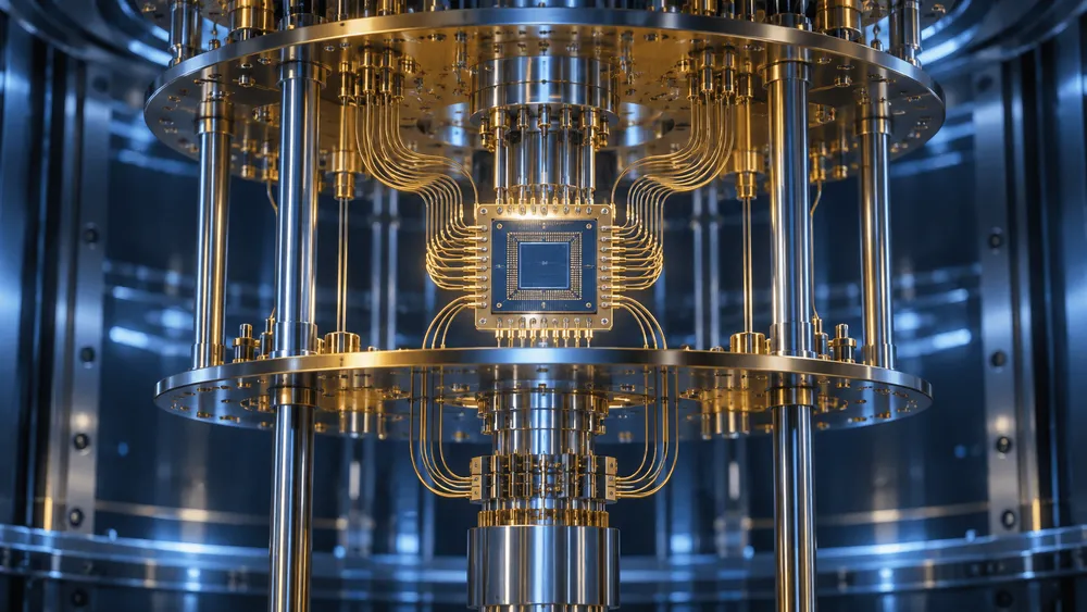
A research team led by Tigran Sedrakyan at US-based BlueQubit has reported obtaining 1 million measurement results from a specific quantum circuit using IBM's "Nighthawk r2" quantum processor, with a QPU runtime of just 19 seconds.
The experiment used a standard execution environment available through a commercial cloud service. According to the team's calculations, generating samples of the same scale and target quality using a specific classical computing method—even on the Frontier supercomputer—would take roughly 110 years.
The findings are summarized in a preprint paper published on September 23, 2026, that has not yet undergone peer review.
However, the figures "19 seconds for a quantum computer versus 110 years for a supercomputer" cannot simply be read as a general measure of computational performance difference.
The 19 seconds is a time actually measured on real quantum hardware, but the 110 years is an estimate derived from a specific classical algorithm and several assumptions. Additionally, how well the 1 million measurement results reproduce the intended probability distribution of the quantum circuit was itself estimated using a separate method.
These three elements need to be considered separately.
1 million measurements on 61 qubits in 19 seconds
The research team used IBM's superconducting quantum processor "Nighthawk r2," which has 120 qubits.
On IBM Quantum, it is offered as ibm_phoenix.
For the experiment, the team selected 61 of these qubits along with 102 connections linking them, and ran a task known as "random circuit sampling."
In random circuit sampling, random operations are repeatedly applied to the qubits, after which all qubits are measured.
In this experiment, each measurement yields a single bit string consisting of 61 digits of 0s and 1s.
However, the goal isn't simply to generate 1 million unrelated random numbers.
A quantum circuit has an inherent distribution describing the probability with which each bit string appears. The challenge is to generate samples that reflect that distribution.
The larger and more complex a quantum circuit becomes, the harder it is for a classical computer to reproduce that probability distribution. For this reason, random circuit sampling has been used as one of the representative benchmarks for comparing the computational power of quantum and classical computers.
That said, this was not an experiment that completed a practical task—such as drug discovery, materials exploration, or code-breaking—in 19 seconds.
In the central experiment, the team repeated a process combining operations on each qubit with CZ gates that entangle qubits together, over 36 cycles.
The entire circuit contained 918 CZ gates.
The QPU runtime used to measure this circuit 1 million times and obtain 1 million 61-bit strings was 19 seconds.
The "19 seconds" is not total wait time on the cloud
The 19 seconds referred to here is the time during which the quantum processor itself was actively used for processing.
It does not represent the real-world elapsed time from when a user submits a job to the cloud, through the queue, to when results are received.
Beyond the main 1-million-sample run, the research team also conducted additional experiments to verify the quality of the circuit.
Combined, the entire experiment involved approximately 9.1 million measurements, with a total QPU runtime of about 11 minutes.
In other words:
- Acquiring the core 1 million samples: 19 seconds
- The entire experiment including quality verification: approximately 11 minutes
These are two distinct figures.
The 19-second figure cannot be interpreted as the total time for the entire research process, including preparation, cloud queue wait times, verification, and data analysis.
No special dedicated tuning was used, but qubits were selected
The experiment used a standard Qiskit cloud environment, without any special hardware calibration dedicated to this benchmark.
This is one notable feature of the result.
On the other hand, the 61 qubits were not randomly chosen from the full set of 120.
The research team examined the standard calibration data provided immediately before the experiment, checking qubit readout errors and single- and two-qubit gate errors, and selected which qubits and connections to use based on that information.
In other words, using hardware accessible to general cloud users is different from running the experiment without regard to the hardware's condition.
Obtaining 1 million samples alone doesn't mean success
Even if 1 million bit strings can be generated quickly, if most of them are essentially noise, it doesn't mean the intended quantum circuit was executed correctly.
So the research team estimated "fidelity"—a measure of how much of the ideal quantum circuit's behavior remains present in the actual hardware's output.
However, they did not directly compare all 1 million results against ideal output probabilities computed by a classical computer for the complete 36-cycle, 61-qubit circuit.
That's because such a calculation is precisely the part described here as "extremely difficult for classical computing."
Instead, they verified quality using two methods with different characteristics.
Splitting the circuit into smaller pieces and comparing to ideal values
The first method is called "patch XEB."
The full 61-qubit circuit is divided into three or four smaller regions.
By removing the CZ gates that span across regions, each resulting circuit becomes small enough that a classical computer can precisely calculate its ideal output probabilities.
Comparing these ideal values against the actual measured results from the hardware is the cross-entropy benchmark (XEB).
The research team prepared five different ways of splitting the circuit for both the three-way and four-way divisions, and additionally ran three types of random circuits for each split.
As a result, each circuit depth evaluation includes 15 different circuits.
However, what this method evaluates is not the actual complete 61-qubit circuit used to obtain the full 1 million samples.
Also checking whether running the circuit backward returns to the original state
The other method is called "mirror benchmarking."
After running a quantum circuit forward, the team continues with reverse operations that cancel out that processing.
On an ideal quantum computer, this would ultimately return to the initial state that was prepared.
On real hardware, errors accumulate along the way, so by observing how close the system gets back to the original state, one can estimate the overall quality of the circuit.
This method does not require calculating the ideal output probability distribution on a classical computer.
The research team performed mirror benchmarking across 4 to 40 cycles, and patch XEB across 20 to 40 cycles.
In the range where both methods were measured, they report that the fidelity values obtained from the two methods closely matched.
At 36 cycles, the directly obtained proxy metric was approximately 1.8–2.2×10^-3, while the value derived by fitting a curve to the overall measurement results was approximately 0.0023.
This 0.0023 does not mean that only 0.23% of the 1 million runs were "correct."
It is a metric representing how much of the quantum circuit's ideal probability distribution remains present in the actual hardware's output.
The fact that two different verification methods produced similar results provides supporting evidence for the fidelity estimate.
However, this does not constitute a direct verification of the entire output distribution for the complete 61-qubit circuit.
The "roughly 110 years on Frontier" is not a measured value
On the other hand, the classical-computing figure of "roughly 110 years" is not an actual measured value.
It is a number derived by the research team estimating the computational workload required for classical simulation, then converting that into terms of Frontier's performance.
The basic method used is called "tensor network contraction."
This represents the quantum circuit as a network of numerous interconnected numerical data points, then combines them in an efficient order to calculate the probability of a specific bit string appearing.
Furthermore, using that probability, they estimated the computational workload for rejection sampling to generate 1 million samples from a distribution corresponding to the fidelity estimated in the experiment.
The paper calculated this workload at approximately 1.2×10^27 operations.
This was then converted using Frontier's theoretical peak performance of 1.685×10^18 floating-point operations per second.
However, the calculation assumes Frontier can sustain only 20% of its theoretical peak performance continuously.
The result of this calculation is approximately 110 years.
The main text of the paper states approximately 110 years, while Table 1 states 108 years—a discrepancy due to different rounding methods.
Assumptions favorable to the classical side were also included
This calculation assumes unlimited access to working memory and ignores internal communication costs within the supercomputer.
In real-world computing systems, memory capacity has limits, and dividing large-scale calculations requires additional processing overhead.
In that sense, this estimate includes some conditions favorable to the classical computer side.
On the other hand, there is uncertainty running in the opposite direction as well.
In tensor networks, the required computational workload can vary dramatically depending on the order in which data is combined.
The research team searched for an efficient calculation order, but did not prove that this represents the mathematically optimal method.
The authors themselves state in the paper:
"All costs presented remain upper bounds on the true optimal contraction cost."
In other words, if a more efficient calculation method is discovered in the future, the roughly-110-year estimate could shrink.
Not "110 years no matter what classical computer is used"
The roughly 110-year figure does not represent a fundamental limit that no classical algorithm could ever surpass.
It is based on the specific tensor network method and sampling approach that the research team evaluated.
The paper mentions several speedup possibilities not fully incorporated into this calculation, including:
- Reusing intermediate calculation results when computing multiple output probabilities
- Using approximate rather than exact tensor contraction
- Utilizing matrix product states (MPS)
- Matching only the XEB score without reproducing the actual distribution
The roughly 110-year figure represents "what this level of effort requires under the specific classical method currently examined," not a mathematical lower bound for classical computation as a whole.
In past research on quantum advantage, there have been cases where, after quantum-side experiments were published, classical simulation methods were subsequently improved, substantially reducing the originally estimated time.
Matching XEB scores and reproducing the same distribution are also different things
Another important point concerns what exactly the classical side is being asked to reproduce.
"Achieving the same XEB score" and "generating samples from a probability distribution with fidelity comparable to the quantum experiment" are not the same task.
The roughly 110-year estimate in this study targets the latter.
Meanwhile, classical methods have also been studied that raise evaluation metrics without reproducing the actual distribution of the real quantum circuit.
To fairly compare speed, one needs to align:
- The number of samples
- The quality of the output
- Which metric is being matched
- Which algorithm is being used
"1 million samples, 19 seconds" was independently reproduced on a public cloud
One notable feature of this research is that third parties can attempt the same experiment.
Sedrakyan and colleagues have published the circuit used, the measured bit strings, and the code for estimating classical computational workload.
The paper, "Quantum computational advantage in random-circuit sampling on IBM superconducting quantum computers," is available as arXiv:2609.28657v1.
At this time, it remains a preprint that has not undergone peer review.
After publication, on September 25, Edukaizen ran the same 61-qubit, 36-cycle circuit on the same ibm_phoenix system using the same physical qubit layout.
They report obtaining 1 million samples with a QPU runtime, as recorded by IBM, also of 19 seconds.
At minimum, this means the following claim has been reproduced by a third party:
"The QPU time required to measure the published circuit 1 million times on Nighthawk r2 is 19 seconds."
However, what Edukaizen reproduced was primarily the circuit execution and timing.
They did not independently re-run all of the patch XEB and mirror benchmarking methods used in the paper to independently confirm the approximately 0.0023 fidelity figure.
Edukaizen's own site explicitly notes this limitation.
Therefore, this does not mean that the entire "quantum advantage" claim has been confirmed through peer-reviewed, independent replication.
What comes next: reproducibility on the quantum side, improvements on the classical side
What was directly confirmed in this experiment is that a 61-qubit, 36-cycle random circuit could be run on Nighthawk r2—accessible through IBM's commercial cloud—and that 1 million outputs could be obtained with 19 seconds of QPU time.
Furthermore, two verification methods with different characteristics produced similar results regarding the circuit's fidelity.
On the other hand, the claim that "a classical computer would take roughly 110 years" is an estimate based on a specific algorithm and specific computational conditions.
Future verification can proceed in two directions.
One is whether third parties running the same quantum circuit can reproduce not just the 19-second speed, but also comparable fidelity results.
The other is testing how fast classical computing methods, using new simulation techniques, can generate 1 million samples of equivalent quality.
What matters most about this result is not simply the striking "19 seconds versus 110 years" comparison.
What matters is that the quantum circuit, measurement data, and code for estimating classical computational workload have all been made public, allowing third parties to verify the results using the same commercial cloud quantum processor.
Will the same quality be reproducibly achieved on the quantum side? And how much can the classical side narrow down that roughly-110-year estimate? Only by accumulating answers to both questions can we properly assess just how strong the quantum computing advantage demonstrated here truly is.